Teradata Partitioned Primary Index (PPI) 

What is the Concept behind Partitioning a Table?

• Each Table in Teradata has a Primary Index unless it is a NoPI table.
• The Primary Index is the mechanism that allows Teradata to physically distribute the rows of a table across the AMPs.
• AMPs Sort their rows by the Row-ID, so the system can perform a lightning fast Binary Search since the rows are in Row-ID Order.
• Partitioning merely tells the AMP to sort its tables’ rows by the Partition first, but then sort the rows by Row-ID within the partition.
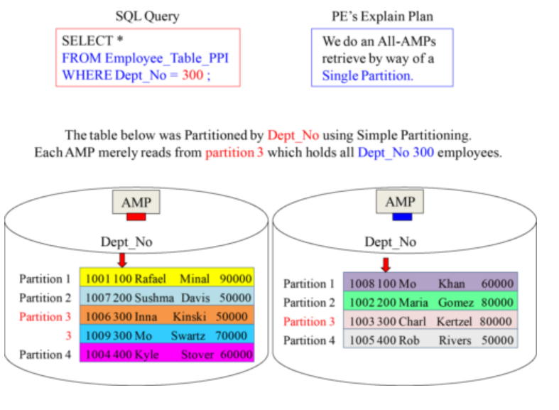
• Partitioning queries will involve all AMPs, but partitioned tables are designed to prevent FULL Table Scans.

Advantages and Disadvantages of Partitioning

Advantages

• Increase query efficiency by avoiding full table scans
• PPI’s are defined on a table in order to increase query efficiency by avoiding full table scans without the overhead and maintenance costs of secondary indexes.
• Deleting large volumes of rows in entire partitions can be extremely fast.
• For range based queries we can effectively remove SI and use PPI, thus saving overhead of SI subtable.
• It can access a subset of a large table quickly.
• Maximum partitions allowed by Teradata – 65,535

Disadvantages

• Partitioned rows are2 or 8 bytes longer. Table uses more PERM space.
• A PI access may be degraded if the partitioning column is not part of the PI
• Joins to non-partitioned tables with the same PI may be degraded.
• The PI can’t be defined as unique when the partitioning column is not part of the PI.

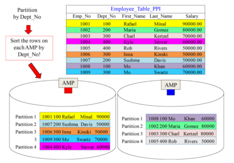
Creating a PPI Table with Simple Partitioning

• A PPI table has the AMPs sort (order) the rows on the table by the Partition.
• This allows for people to avoid Full Table Scans.

A Visual Display of Simple Partitioning

An SQL Example that explains Simple Partitioning

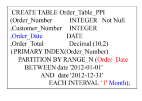
Creating a PPI Table with RANGE_N

• The expression is evaluated and is mapped into one of a list of specified ranges.
• Ranges are listed in increasing order and must not overlap with each other.
• Result is the data row being placed into a partition associated with that range.

Examples:

Example 1 – Creating a PPI Table with RANGE_N Partitioning per Month

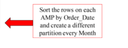
A Visual of One Year of Data with Range_N per Month

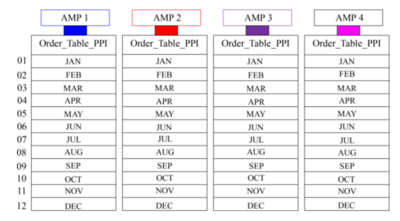
Each AMP sorts their rows by Month (of Order_Date).

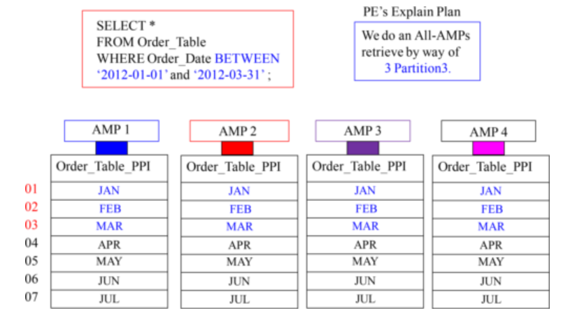
An SQL Example explaining Range_N Partitioning per Month

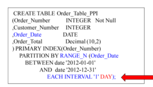
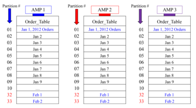
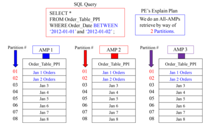
Example 2 – Creating a PPI Table with RANGE_N Partitioning per Day

A Visual of Range_N Partitioning Per Day

An SQL Example that explains Range_N Partitioning per Day

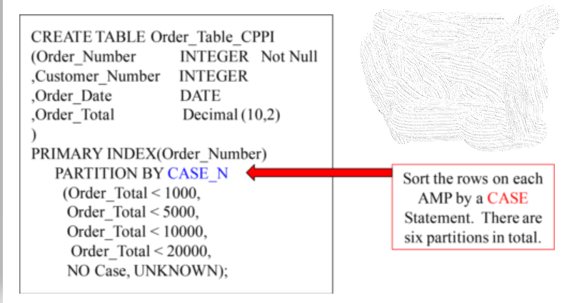
Creating a PPI Table with CASE_N

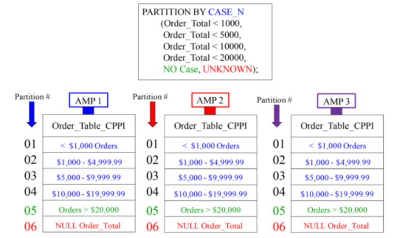
A Visual of Case_N Partitioning

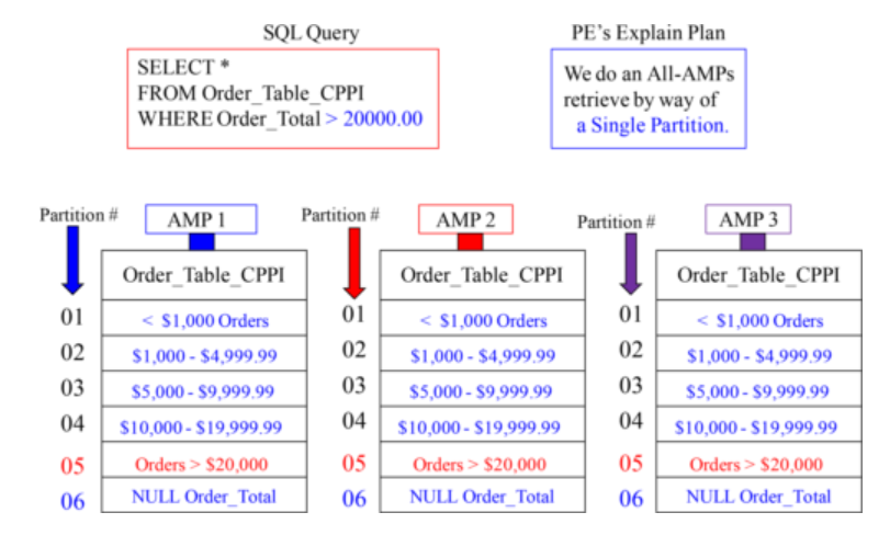
An SQL Example that explains CASE_N Partitioning

Note: NO CASE, NO RANGE, and UNKNOWN options are also available which we can use in RANGE_N and CASE_N Partitioning